Description

CMD contains hundreds of thousands of 2D maps and 3D grids created from cosmological simulations run with different codes. The CMD data is arranged into different files whose name indicate the properties of the simulations used to generate it. This is because the CMD data, as CAMELS, can be classified into into suites and sets (see this page for what concerns the CAMELS simulations):

Suites

CMD has been generated from thousands of state-of-the-art (magneto-)hydrodynamic and gravity-only N-body simulations from the CAMELS project. CMD data can be classified into different suites, that indicate the type of simulation used to create the data:

IllustrisTNG. These magneto-hydrodynamic simulations follow the evolution of gas, dark matter, stars, and black-holes. They also simulate magnetic fields. CMD uses 1,088 of these simulations.
SIMBA. These hydrodynamic simulations follow the evolution of gas, dark matter, stars, and black-holes. CMD uses 1,088 of these simulations.
Astrid. These hydrodynamic simulations follow the evolution of gas, dark matter, stars, and black-holes. CMD uses 1,088 of these simulations.
N-body. These gravity-only N-body simulation only follow the evolution of dark matter. Thus, they do not model astrophysical processes such as the formation of stars and the feedback from black-holes. There is an N-body simulation for each (magneto-)hydrodynamic simulation. CMD uses 2,000 of these simulations.

Sets

Each suite contains different sets, that indicate how the value of the labels of the underlying simulations are organized:

CV. The value of the labels is always the same and correspond to the fiducial model. The 2D maps and 3D grids only differ on the initial conditions of the simulations run. This set contains 27 simulations.
1P. The value of the labels is varied one-at-a-time. I.e. the 2D maps and 3D grids have labels whose value only differ in one element from the value of the fiducial maps (CV set). In this case, the initial conditions are always the same. This set contains 61 simulations.
LH. The value of all labels is different in each simulation and the values are organized in a latin-hypercube. The value of the initial conditions is different in each simulation. This set contains 1,000 simulations.
EX. The value of the labels is chosen to be extreme and the initial conditions of the simulations are the same. This set contains 4 simulations.
BE. The underlying simulations have the same initial conditions and the same value of the labels (the fiducial ones). The only difference between the simulations is due to random noise from numerical approximations. This set contains 27 simulations. So far, this set is only present for the IllutrisTNG suite.

Attention

When working with CMD data, you will use files whose name will indicate the suite and the set. For instance, the file Maps_Mcdm_Astrid_1P_z=0.00.npy contains 2D maps of the cold dark matter field created from Astrid 1P simulations. In other workds, the simulations have been run with the Astrid model and their parameters follow the 1P configuration: all simulations have the same initial conditions but their parameters only vary from those of the fiducial ones in a single parameter.

Structure

CMD provides the following data generated from the above simulations:

IllustrisTNG

16,785 2D maps per field for 13 different fields. 218,205 2D maps in total.
16,380 3D grids per field for 13 different fields. 212,940 3D grids in total.

SIMBA

16,380 2D maps per field for 12 different fields. 196,560 2D maps in total.
16,380 3D grids per field for 12 different fields. 196,560 3D grids in total.

Astrid

16,380 2D maps per field for 12 different fields. 196,560 2D maps in total.
16,380 3D grids per field for 12 different fields. 196,560 3D grids in total.

Nbody

49,140 2D maps of one single field. 49,140 2D maps in total.
49,140 3D grids of one single field. 49,140 3D grids in total.

The table summarizes the properties of the 2D maps:

Field	Prefix	IllustrisTNG	SIMBA	Astrid	Nbody	Units
		Number of 2D maps
Gas density	Mgas	16,785	16,380	16,380	–	\((M_\odot/h)/({\rm Mpc}/h)^2\)
Gas velocity	Vgas	16,785	16,380	16,380	–	km/s
Gas temperature	T	16,785	16,380	16,380	–	Kelvin
Gas pressure	P	16,785	16,380	16,380	–	\(h^2M_\odot{\rm (km/s)^2/kpc^3}\)
Gas metallicity	Z	16,785	16,380	16,380	–	dimensionless
Neutral hydrogen density	HI	16,785	16,380	16,380	–	\((M_\odot/h)/({\rm Mpc}/h)^2\)
Electron number density	ne	16,785	16,380	16,380	–	\(h^2/{\rm cm}^3({\rm Mpc}/h)\)
Magnetic fields	B	16,785	–	–	–	Gauss
Magnesium over Iron	MgFe	16,785	16,380	16,380	–	dimensionless
Dark matter density	Mcdm	16,785	16,380	16,380	–	\((M_\odot/h)/({\rm Mpc}/h)^2\)
Dark matter velocity	Vcdm	16,785	16,380	16,380	–	km/s
Stellar mass density	Mstar	16,785	16,380	16,380	–	\((M_\odot/h)/({\rm Mpc}/h)^2\)
Total matter density	Mtot	16,785	16,380	16,380	49,140	\((M_\odot/h)/({\rm Mpc}/h)^2\)

Total		218,205	196,560	196,560	49,140

The table summarizes the properties of the 3D grids:

Field	Prefix	IllustrisTNG	SIMBA	Astrid	Nbody	Units
		Number of 3D grids
Gas density	Mgas	16,380	16,380	16,380	–	\((M_\odot/h)/({\rm Mpc}/h)^3\)
Gas velocity	Vgas	16,380	16,380	16,380	–	km/s
Gas temperature	T	16,380	16,380	16,380	–	Kelvin
Gas pressure	P	16,380	16,380	16,380	–	\(h^2M_\odot{\rm (km/s)^2/kpc^3}\)
Gas metallicity	Z	16,380	16,380	16,380	–	dimensionless
Neutral hydrogen density	HI	16,380	16,380	16,380	–	\((M_\odot/h)/({\rm Mpc}/h)^3\)
Electron number density	ne	16,380	16,380	16,380	–	\(h^2/{\rm cm}^3\)
Magnetic fields	B	16,380	–	–	–	Gauss
Magnesium over Iron	MgFe	16,380	16,380	16,380	–	dimensionless
Dark matter density	Mcdm	16,380	16,380	16,380	–	\((M_\odot/h)/({\rm Mpc}/h)^3\)
Dark matter velocity	Vcdm	16,380	16,380	16,380	–	km/s
Stellar mass density	Mstar	16,380	16,380	16,380	–	\((M_\odot/h)/({\rm Mpc}/h)^3\)
Total matter density	Mtot	16,380	16,380	16,380	49,140	\((M_\odot/h)/({\rm Mpc}/h)^3\)

Total		212,940	196,560	196,560	49,140

where \(M_\odot\) represents the mass of the Sun, km/s stands for kilometers per second, \(h\) is the reduced Hubble constant, that in all CMD is fixed to 0.67, and \({\rm kpc}\) stands for kiloparsec (3,260 light years). The coefficient \(A\) is 2 for 2D maps and 3 for 3D grids.

Warning

We note that some of the units reported in the CMD paper (see Table 1) are not correct. The units for the electron density are missing several factors and the pressure units lacks a \(h^2\) factor. The above table shows the correct units of the 2D maps and 3D grids.

Note

All 2D maps have \(256^2\) pixels and cover a periodic area of \((25~h^{-1}{\rm Mpc})^2\) at redshift 0. The 3D grids contain \(128^3\), \(256^3\) or \(512^3\) voxels over a volume of \((25~h^{-1}{\rm Mpc})^3\) and are at redshifts 0, 0.5, 1, 1.5, and 2.

We show an example of how the IllustrisTNG images look like for the different fields:

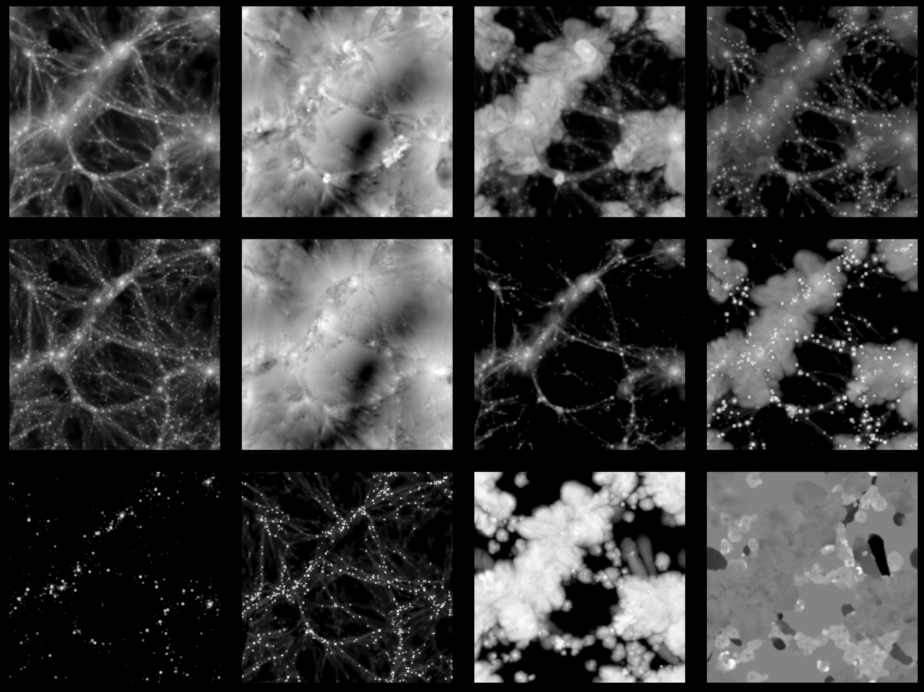
where from top-left to bottom-right: gas density, gas velocity, gas temperature, gas pressure, dark matter density, dark matter velocity, electron number density, magnetic fields, stellar mass density, neutral hydrogen mass density, gas metallicity, and magnesium over iron ratio.

These images show different properties of the gas, dark matter, and stars in a given Universe. Determining the value of the cosmological parameters from these images will help us to decode the true value of our own Universe, allowing us to unveil some of the biggest mysteries in fundamental physics.

Labels

Each 2D map and 3D grid has a set of labels attached to it:

\(\Omega_{\rm m}\). This is a cosmological parameter that represents the fraction of matter in the Universe.
\(\sigma_8\). This is a cosmological parameter that controls the smoothness of the distribution of matter in the Universe.
\(A_{\rm SN1}\) and \(A_{\rm SN2}\). These are two astrophysical parameters that controls two properties of supernova feedback.
\(A_{\rm AGN1}\) and \(A_{\rm AGN2}\). These are two astrophysical parameters that control two properties of black-hole feedback.

The data from the IllustrisTNG, SIMBA, and Astrid simulations are described by all the above parameters, while the 2D maps and 3D grids generated from the N-body simulations are only characterized by the cosmological parameters \(\Omega_{\rm m}\) and \(\sigma_8\).

2D maps

The generic name of the files containing the maps is Maps_prefix_suite_set_z=0.00.npy, where prefix is the word identifying each field (see table above), suite is the suite (IllustrisTNG, SIMBA, Astrid, Nbody_IllustrisTNG, Nbody_SIMBA, or Nbody_Astrid) and set is the set (1P, CV, LH).

Note

In the case of the Nbody data we add an extra word, IllustrisTNG, SIMBA, or Astrid, to characterize the matching data from the (magneto-)hydrodynamics simulations. See Matching data for further details.

For instance, the file containing the gas density maps of the IllustrisTNG simulations is Maps_Mgas_IllustrisTNG_LH_z=0.00.npy. The 2D maps are stored as .npy files, and can be read with the numpy load routine. For instance, to read the SIMBA gas temperature maps do:

import numpy as np

# name of the file
fmaps = 'Maps_T_SIMBA_LH_z=0.00.npy'

# read the data
maps = np.load(fmaps)

The file contains 15,000 maps with \(256^2\) pixels each.

We note that the name of the files for the Nbody 2D maps is slighty different to reflect the (magneto-)hydrodynamic simulation they should be matched on:

The values of the cosmological and astrophysical parameters characterizing the maps of a given field are given in params_sim.txt where suite can be IllustrisTNG, SIMBA, Astrid, or Nbody. These files can be read as follows:

import numpy as np

# name of the file
fparams = 'params_SIMBA.txt'

# read the data
params = np.loadtxt(fparams)

The file contains 1,000 entries with 6 values per entry. The first and second entries are the values of \(\Omega_{\rm m}\) and \(\sigma_8\), while the rest represent the values of the astrophysical parameters: \(A_{\rm SN1}\), \(A_{\rm AGN1}\), \(A_{\rm SN2}\), \(A_{\rm AGN2}\).

Note

In the case of the Nbody maps, only the first and second columns (the ones containing the values of \(\Omega_{\rm m}\) and \(\sigma_8\)) are relevant. The other 4 columns can be disregarded (because the Nbody simulations do not model supernovae and black holes). They are only kept to standardize the training of the networks.

The values of the cosmological and astrophysical parameters of a given map can be found as

map_number = 765
params_map = params[map_number//15]

See this colab for further details on how to manipulate the images and the values of the parameters.

Note

2D maps can be generated from 3D grids by taking slides and projecting along a given axis. See this colab for an example.

3D grids

The generic name of the files containing the 3D grids is Grids_prefix_suite_set_grid_z=redshift.npy, where prefix is the word identifying each field (see table above), suite can be IllustrisTNG, SIMBA, Astrid, Nbody_IllustrisTNG, Nbody_SIMBA or Nbody_Astrid, set can be 1P, CV, LH, grid can be 128, 256, or 512 and redshift can be 0, 0.5, 1, 1.5 or 2.

Note

In the case of the Nbody data we add an extra word, IllustrisTNG, SIMBA or Astrid, to characterize the matching data from the (magneto-)hydrodynamics simulations. See Matching data for further details.

For instance, the file containing the 3D gas metallicity of the IllustrisTNG simulations on a grid with 256^3 voxels at redshift 0 is Grids_Z_IllustrisTNG_LH_256_z=0.00.npy. The 3D grids are stored as .npy files, and can be read with the numpy load routine. For instance, to read the SIMBA neutral hydrogen mass density at redshift 1.0 with a grid of 128^3 voxels do:

import numpy as np

# name of the file
fgrids = 'Grids_HI_SIMBA_LH_128_z=0.00.npy'

# read the data
grids = np.load(fgrids)

The file contains 1,000 grids with \(128^3\) voxels each. For large files (e.g. those containing the grids with \(512^3\) voxels) it is better to read the files in a slightly different way, to avoid running out of RAM memory:

import numpy as np

# name of the file
fgrids = 'Grids_Mcdm_Nbody_LH_512_z=0.00.npy'

# read the data
grids = np.load(fgrids, mmap_mode='r')

# take the first 3D grid
grids[0]

# multiply all the grids from numbers 672 to 700 by 3
grids[672:700]*3

The values of the cosmological and astrophysical parameters characterizing the maps of a given field can be found in params_set_suite.txt where suite can be IllustrisTNG, SIMBA, Astrid, or Nbody, and set can be 1P, CV, or LH. These files can be read as follows:

import numpy as np

# name of the file
fparams = 'params_LH_SIMBA.txt'

# read the data
params = np.loadtxt(fparams)

The file contains 1,000 entries with 6 values per entry. The first and second entries are the values of \(\Omega_{\rm m}\) and \(\sigma_8\), while the rest represent the values of the astrophysical parameters: \(A_{\rm SN1}\), \(A_{\rm AGN1}\), \(A_{\rm SN2}\), \(A_{\rm AGN2}\).

Note

In the case of the Nbody maps, only the first and second columns (the ones containing the values of \(\Omega_{\rm m}\) and \(\sigma_8\)) are relevant. The other 4 columns can be disregarded (because the Nbody simulations do not model supernovae and black holes). They are only kept to standardize the training of the networks.

The value of the cosmological and astrophysical parameters of a given grid can be found as

grid_number = 821
params_map  = params[map_number]

Symmetries

Each 2D map and 3D grid from CMD has a set of labels associated to it: two cosmological parameters and four astrophysical parameters (only in the case of data from IllustrisTNG, SIMBA, and Astrid simulations). These labels will remain the same if

rotations
translations
parity

transformations are applied to the data. Another important thing to take into account is that the data is periodic in all dimensions. For instance, in the case of 2D maps

import numpy as np

# name of the file
fmaps = 'Maps_HI_IllustrisTNG_LH_z=0.00.npy'

# read the data
maps_HI = np.load(fmaps)

# take the map number 36
map_HI = maps_HI[36]

# the pixel map_HI[45,89] is adjacent to the pixel map_HI[46,89]
# the pixel map_HI[145,99] is adjacent to the pixel map_HI[145,98]
# the pixel map_HI[76,0] is adjancent to the pixel map_HI[76,255]
# the pixel map_HI[255,12] is adjancent to the pixel map_HI[0,12]

Note

When using convolutional neural networks, one can take advantage of this property by using periodic padding.

Matching data

There are several ways to match CMD.

The 2D maps and 3D grids can be matched across fields within the same simulation type. For instance, the maps number 2786 of the files Maps_ne_IllustrisTNG_LH_z=0.0.npy and Maps_B_IllustrisTNG_LH_z=0.0.npy represent the same region of the same simulation. The only difference is that the first map will show the electron abundance while the second shows the magnetic fields. The same thing applies to the 3D grids. For instance, the grids number 621 of the files Grids_HI_SIMBA_LH_128_z=0.0.npy and Grids_Mgas_SIMBA_LH_128_z=0.0.npy represent the same volume of the same simulation with the only difference that the first grid shows the neutral hydrogen mass density while the second contains the gas density.

Warning

This matching only applies to data within the same simulation. E.g. the files Maps_Mcdm_IllustrisTNG_LH_z=0.0.npy do not have any correspondence with the maps in the file Maps_Mtot_SIMBA_LH_z=0.0.npy.

The 3D grids can be matched across resolution within the same field and redshift. For instance, the grids number 167 of the files Grids_Vcdm_SIMBA_LH_128_z=1.0.npy and Grids_Vcdm_SIMBA_LH_256_z=1.0.npy represent exactly the same field over the same volume with the only difference that the first contains \(128^3\) voxels while the second has \(256^3\) voxels. Knowing this mapping is important for the Superresolution application.
The 2D maps and 3D grids can be matched between (magneto-)hydrodynamic and N-body simulations. For instance, the maps number 7413 of the files Maps_Mtot_IllustrisTNG_LH_z=0.0.npy and Maps_Mtot_Nbody_IllustrisTNG_LH_z=0.0.npy represent the same region of the same field (total matter), with the only difference that the first map was generated from an IllustrisTNG magneto-hydrodynamic simulation while the second one is from a gravity-only N-body simulation. Knowing this mapping is important to be able to quantify that impact of astrophysical processes on a given task.

Warning

This mapping only applies to the total matter field.

The 3D grids can be matched across cosmic time in both the (magneto-)hydrodynamic and the N-body simulations. For instance, the grids number 923 Grids_Vgas_SIMBA_LH_512_z=0.0.npy and Grids_Vgas_SIMBA_LH_512_z=2.0.npy represent the gas velocity of the same universe just at two different times: \(z=0\) in the first grid and \(z=2\) in the second grid.

Note

We do not recommend using the above time matching for the 2D maps. The reason is that in a simulation, particles will move with time, so particles that are in a given map at a given time may move to another map at a different time. While this is not a problem for the 3D grids, it may be a challenge for the 2D maps.

We note that the above three matchings can be combined. For instance, in the N-body to hydro application we want to find the mapping between the total matter from an N-body simulation and a given field from a (magneto-)hydrodynamic simulation. In this case, the grids number 714 of the files Grids_T_SIMBA_LH_256_z=0.0.npy and Grids_Mtot_Nbody_SIMBA_LH_256_z=0.0.npy represent the same region at redshift 0, the first grid will contain the gas temperature from the hydrodynamic simulation while the second is the total matter field from the equivalent N-body simulation.

Storage

Each pixel of a 2D map and each voxel of a 3D grid is stored as a float, i.e. it occupies 4 bytes.

A single 2D map that has \(256^2\) pixels will take \(256^2\times4=0.25\) Mb. CMD is organized into files that contain different number of maps. For instance, the files of the LH set contain 15,000 maps per field. Each of those files would thus require 3.75 Gb. If you want to download all the maps of the IllustrisTNG LH set (13 different fields) you would need ~50 Gb.

A single 3D grid with \(N^3\) voxels will take \(N^3\times4\) bytes, i.e. 8 Mb for \(N=128\), 64 Mb for \(N=256\), or 512 Mb for \(N=512\). CMD is organized into files that contain different numbers of 3D grids. For instance, the files of the LH sets contain 1,000 grids. Each of those LH files will occupy 7.8 Gb (\(N=128\)), 62.5 Gb (\(N=256\)), and 500 Gb (\(N=512\)). If you want to download all 12 grids of the LH set for SIMBA at \(N=512\) it will require ~6 Tb.